Users guide¶

Installation¶

There is no special installation required. It can be downloaded from https://github.com/vondrejc/FFTHomPy.git or using Git by:

git clone https://github.com/vondrejc/FFTHomPy.git

The code is implemented in python and supports versions 2 and 3.

The software also requires the following numerical libraries:

numpy
scipy

Running the program¶

Command line usage:

$ python main.py examples/scalar/scalar_2d.py

or only as:

$ ./main.py examples/scalar/scalar_2d.py

where examples/scalar/scalar_2d.py is an input file for FFTHomPY.

Definition of input file¶

Input file for FFTHomPy consists of material definition and problem definition.

Material definition¶

Material coefficients can be defined as matrix-inclusion composites or grid-based composites.

Matrix-inclusions composites¶

In this case, material is expressed at points $\Vx$ of periodic cell $\puc=\prod_{i=1}^d (-\frac{Y_i}{2},\frac{Y_i}{2})$ as

$\TA(\Vx) &= \sum_{i=1}^n f\incl{i} (\Vx-\Vx\incl{i}) \TA\incl{i}$

where functions $f\incl{i}$ describe inclusion topologies located at $\Vx\incl{i}$ with material coefficients $\TA\incl{i}\in\xRdd$ . An example of material coefficients is named 'square'

import numpy as np

materials = {'square': {'Y': np.ones(dim),
                        'inclusions': ['square', 'otherwise'],
                        'positions': [np.zeros(dim), ''],
                        'params': [0.6*np.ones(dim), ''],
                        'vals': [11*np.eye(dim), 1.*np.eye(dim)]}}

and the used keywords have following meanings:

'Y': numpy.array of shape (dim,) describes the size of periodic cell $\puc$ in dimension dim

'inclusions': list of inclusions $f\incl{i}$ of following types

'square', 'circle', and 'otherwise' in two-dimensional settings

'cube', 'ball', and 'otherwise' in two-dimensional settings

'positions': list of positions $\Vx\incl{i}$ corresponding to individual inclusions

the position corresponds to center of gravity with respect to coordinate system; the inclusion 'otherwise' has no position because it represents the area in periodic cell omitted by inclusions

'params': list of parameters determining the inclusions

for 'square' and 'cube', it corresponds to sizes of individual sides

for 'circle' and 'ball', it corresponds to diameter

'vals': list of material coefficients for individual inclusions; coefficients are represented as numpy.array of shape corresponding to physical problem according to problem definition; for scalar elliptic problem, the shape is (dim, dim) while for linearized elasticity the shape is (D, D) where D = dim*(dim+1)/2.

Grid-based composites¶

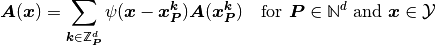
Contrary to Matrix-inclusions composites, grid-based composites are defined on grid points:

$\xPk = \sum_{\alp} \frac{Y_{\alp}k_{\alp}}{P_{\alp}} \cb{\alp}\quad \text{for } \Vk \in \ZPd = \biggl\{ \Vk \in \set{Z}^d : -\frac{P_\alpha}{2} \leq k_\alpha < \frac{P_\alpha}{2} \biggr\}$

for some number of points $\VP\in\xNd$ and the size $\VY\in\xRd$ of periodic cell $\puc=\prod_{i=1}^d (-\frac{Y_i}{2},\frac{Y_i}{2})\subset\xRd$ ; examples for odd and even grids are depicted in following figure

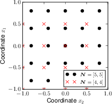
for periodic cell $\puc=\prod_{i=1}^d (-1,1)$ with the cell size $\VY=(2,2)$ .

The material is then approximated with the following formula

(1) $\TA(\Vx) &= \sum_{\Vk\in \set{Z}^d_{\VP}} \psi(\Vx-\Vx^{\Vk}_{\VP}) \TA(\Vx_{\VP}^{\Vk}) \quad\text{for }\VP\in\xNd \text{ and } \Vx\in\puc$

where function $\psi:\puc\rightarrow\xRd$ is taken either by

(2) $\rect_{\Vh}(\Vx) &= \begin{cases} 1 & \text{if } |x_\alp| < \frac{h_\alp}{2}\text{ for all }\alp \\ 0 & \text{otherwise} \end{cases} \quad\text{for }\Vh=\left(\frac{Y_\alp}{P_\alp}\right)_{\alp=1}^d$

leading to piece-wise constant approximation of material coefficients, or by

(3) $\tri_{\Vh}(\Vx) &= \prod_{\alp}\max\{1-|\frac{x_\alp}{h_\alp}|,0\} \quad\text{for }\Vh=\left(\frac{Y_\alp}{P_\alp}\right)_{\alp=1}^d$

leading to piece-wise bilinear approximation of material coefficients.

In comparison to Matrix-inclusions composites, the material coefficients definition

materials.update({'square_Ga': {'Y': np.ones(dim),
                                'inclusions': ['square', 'otherwise'],
                                'positions': [np.zeros(dim), ''],
                                'params': [0.6*np.ones(dim), ''],
                                'vals': [11*np.eye(dim), 1.*np.eye(dim)],
                                'order': 0,
                                'P': 5*np.array(dim)}})

contains two additional parameters:

'P': numpy.array of shape (dim,) describes the resolution of approximation in (1)
'order': define approximation order:
- 0: constant approximation according to (2)
- 1: bilinear approximation according to (3).

Problem definition¶

Here, the example of problem description is stated:

problems = [{'name': 'prob1',
             'physics': 'scalar',
             'material': 'square',
             'solve': {'kind': 'GaNi',
                       'N': N,
                       'primaldual': ['primal', 'dual']},
             'postprocess': [{'kind': 'GaNi'},
                             {'kind': 'Ga',
                              'order': None},
                             {'kind': 'Ga',
                              'order': 0,
                              'P': N},
                             {'kind': 'Ga',
                              'order': 1,
                              'P': 27*N}],
             'solver': {'kind': 'CG',
                        'tol': 1e-6,
                        'maxiter': 1e3}}]

The individual keywords are explained:

'name': the name of a problem
'physics': defines the physical problem that is solved; following alternatives are implemented:
- 'scalar': scalar linear elliptic problem (diffusion, stationary heat transfer, or electric conductivity)
- 'elasticity': linearized elasticity (small strain)
'material': keyword refering to dictionary materials or directly dictionary defining the material coefficients
'solve': defines the problem discretization, the way how to solve minizers (corrector functions)
- 'kind': is either 'Ga' (Galerkin approximation) or 'GaNi' (Galerkin approximation with numerical integration); it thus corresponds to the discretizaiton way
- 'N': is a numpy.array defining the approximation order of trigonometric polynomials; the higher the value is, the better approximation is provided
- 'primaldual': determine if primal, dual, or both formulations are calculated
'solver': defines the linear solver and relating parameters
- 'kind': linear solver one of 'CG' for Conjugate gradients, 'BiCG' for Biconjugate gradients, 'richardson' for Richardson’s iterative solution, 'scipy_cg' for scipy.sparse.linalg.cg, and 'scipy_bicg' for scipy.sparse.linalg.bicg,
- 'tol': the required tolerance (float) for the convergence of linear solver
- 'maxit': the maximal number of iterations
'postprocess': defines the way for calculating homogenized material coefficients from minimizers that are obtained with a way defined in 'solver'
- 'kind': is either 'Ga' (Galerkin approximation) or 'GaNi' (Galerkin approximation with numerical integration); it thus corresponds to the discretizaiton way
- 'order': applicable only for 'Ga', it defines approximation order according to (2) or (3)
- 'P': applicable only for 'Ga', this numpy.array of shape (dim,) describes the resolution of approximation in (1)